Jupyter Notebooks!

I've enjoyed getting re-acquainted with Jupyter Notebooks, which are a great way to 'walk through' an analysis of data, or just how to get, process, transform, map, or otherwise logically work through a problem. Most commonly Jupyter is used with Python and Pandas, but really it can be used with several languages.

This very simple Jupyter workbook is just the result of walking through a tutorial in order to jog the old memory before I dived in with an step by step notebook to show how TextFSM can be used to parse text files to pull out key datapoints from unstructured data. I used this at work to show how we can parse Cisco IOS-XR and Juniper JUNOS output. Send me a note if you'd like to see more on TextFSM.

Video Game Sales

I've created the workbook and stored it in my gitlab account, along with my data source, a list of video game titles and sales over the past few decades.

Optional: Install Anaconda

If you're going to make your own notebooks, you're going to need jupyter installed locally. Head over to anaconda.com and find the instructions for your OS. For me, it was as simple as running brew install anaconda on my mac.

Open the notebook

If you decided to install anaconda locally, first download the VideoGameSales.ipynb jupyter notebook file, and run jupyter notebook in the directory you saved the file.

If you'd prefer to try this out without installing anything, you can open the VideoGameSales.ipynb jupyter notebook in a new window on mybinder.org:

NOTE: mybinder times out if you aren't using it. If this happens to you, simply click the link above to start over.

If you simply click on the ⏯ Run button, the notebook will attempt to run the python in each cell of the notebook, sequentially. I recommend you DON'T do that though, and instead step through it cell by cell, and take a look at what is going on. If you click on the cell first, and then press CTRL-ENTER, it will run the code in that one cell only.

!pip install pandas matplotlib seaborn

This first cell installs a few python modules that we'll import. More on that in a moment. After running this cell, go ahead and click on the next, and press CTRL-ENTER again to run that cell. You'll first notice the In [ ]: to the left of the cell change to In [*]: while it is running and then the asterisk is replaced with a number when it is complete. The number helps you know which cells were completed in which order (yes, you can run or rerun them out of order. Keep in mind that information is 'stored' in memory though, and if the cell you are running depends on something being done before that, it won't work unless you run the predecessor first).

import io
import pandas as pd
import matplotlib.pyplot as plt
import seaborn as sns
import requests
sns.set(style="darkgrid")
source_data_url='https://gist.githubusercontent.com/jrogers512/cee93b2940fbaf4e7ca3f2677bcb81c4/raw/3d176e96d73438b33c49a982d6d4c3561ba9d74a/video-game-sales.csv'
df = pd.read_csv(io.StringIO(requests.get(source_data_url).content.decode('utf-8')))

The first cell includes some imported modules. Pandas is a great library that helps us create 'dataframes' which is python speak for tables, and do some cool things with them like analytics, sorting, graphing, and... just about anything you can think of that a spreadsheet can do. matplot and seaborn are all about graphing. Requests allows us to fetch the csv file via https.

Next, we grab some data about video game sales from a csv file. If you take a look at the csv file, you'll see that it has a ranked list of video games, the release year, genre, publisher and sales information. We store this data in a pandas dataframe. Think of a dataframe as a worksheet in excel. Perfect place to store the contents of a CSV file.

df.head()
df.tail()

The dataframe df has some functions on it. Assuming you have already run the first cell by clicking on it and pressing CTRL-ENTER, you can 'insert' a new cell by clicking on the + icon, and then type in dir(df) in the cell and run it to see all the methods for this dataframe object. If you want to see more details on one of the methods, run a cell with help(df.methodname) in it. .head and .tail are two of the methods. As you might expect, head shows us the first few rows, and tail shows us that last few rows. Give each one a try. Try editing the df.head() cell to show a few more rows by changing it to df.head(15) and re-running the cell.

Since I am primarily interested in global sales and not any of the regional sales numbers, lets drop those columns entirely and store the resulting table in df with df = df.drop(columns=['NA_Sales', 'EU_Sales', 'JP_Sales', 'Other_Sales']). Rerun the df.head() cell to see the global sales are the only remaining sales figures.

Let's rename the column headers while we're here by using the the df.columns method: df.columns = ['Rank', 'Game Title', 'Platform', 'Year', 'Genre', 'Publisher', 'Sales (in Billions)']

Click on the df.tail() cell, and rerun it to see the new header names.

Try the len(df) cell to see how many rows are in the dataframe.

Dataframe columns are 'typed' similar to what you'd find in a database (or spreadsheet). Lets see what each column type is currently by running the df.dtypes cell.

Rank            int64
Game Title     object
Platform       object
Year          float64
Genre          object
Publisher      object
Sales         float64
dtype: object

This all looks pretty good, except the Year column. I noticed in the earlier head() output that Wii Sports came out in 2006.0. I would prefer the Year to be an Integer, not a float, however converting it to Integer is not natively possible in Pandas currently if there are null values in the column. Let's see if there are null values in this column before converting it to an Integer.

len(df[df.Year.isnull()]) reveals there are 271 out of 16598. A bit more than 1.5% of our records don't have a release year. Are there a lot of null values in this set? Lets count all null values in all columns. len(df[df.isnull().any(axis=1)]) shows 307 total. Sounds like the Year column is worst offender. I guess I won't convert to integer, and just be annoyed each time I see .0 attached to a year. meh.

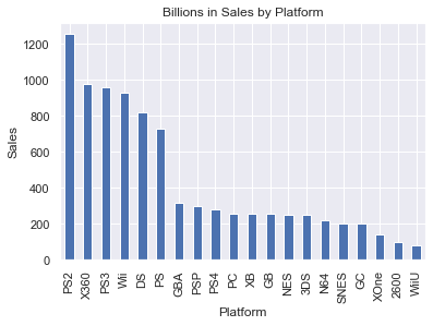
Let's see look at sales by platform. df.groupby("Platform")["Sales"].sum().sort_values(ascending=False).head() does a groupby on Platform, which essentially aggregates all the Sales by Platform. We add up the sales, then sort in descending order, then just look at the top grossing platforms. in a bar chart by using the .plot.bar() method.

Cool. How about sales by year? Was there a 'boom era' for video games? We'll do the same thing, but groupby Year. This time we'll use a line graph.

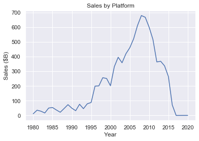
Looks like the peak of video game sales was around 2007. If I were more ambitious, I'd overlay market data to see if the trend of video game sales is congruent with stock market capitalization.

Conclusion

Out of all of this interesting data, I'm reminded of a few things. First of all, pandas is one slick library, which makes slicing/dicing tabular data really convenient. Rarely do I need a loop/lamda/recursion to do something with a what could be a ton of data. So much easier to think about data when you don't get lost in a recursion. Second, jupyter notebooks are a really great way of documenting your code, or an idea, and stepping through it as a prototype. It is useful to teach others about how to do something, and even more useful for 'remembering' how something you did a while ago works.

Lastly... using mybinder is kind of rough. Constant disconnects, and performance is kind of painful. Instead I recommend running jupyter locally using anaconda.

I hope you enjoyed this walkthrough of jupyter and pandas. Send me a note with any questions or comments!